Experiment 11: Measuring a human hair

Introduction

                The purpose of this experiment is to measure a human hair using the concepts of light interference. This experiment was conducted using a human hair, a 3x5 notecard, a whiteboard, and a microscope. A human hair was taped across a hole in 3x5 notecard, and let it parallel to the whiteboard at a known distance. A laser was used to point toward the white board through the hair. The distance between the first 2 fringes was recorded. The diameter of the human hair was measured experimentally using a micrometer, and this result was compared with the actual diameter of the hair. The theoretical result was computed using

d=λL/y

where d= diameter of the hair

λ= wavelength of the laser

L= Distance between the laser and the whiteboard

y= distance between 2 adjacent diffraction pattern.

Figure 1: A laser beam perpendicular to the axis passing through the hair

Figure 2: Diffraction pattern formed by the laser beam due to light interference

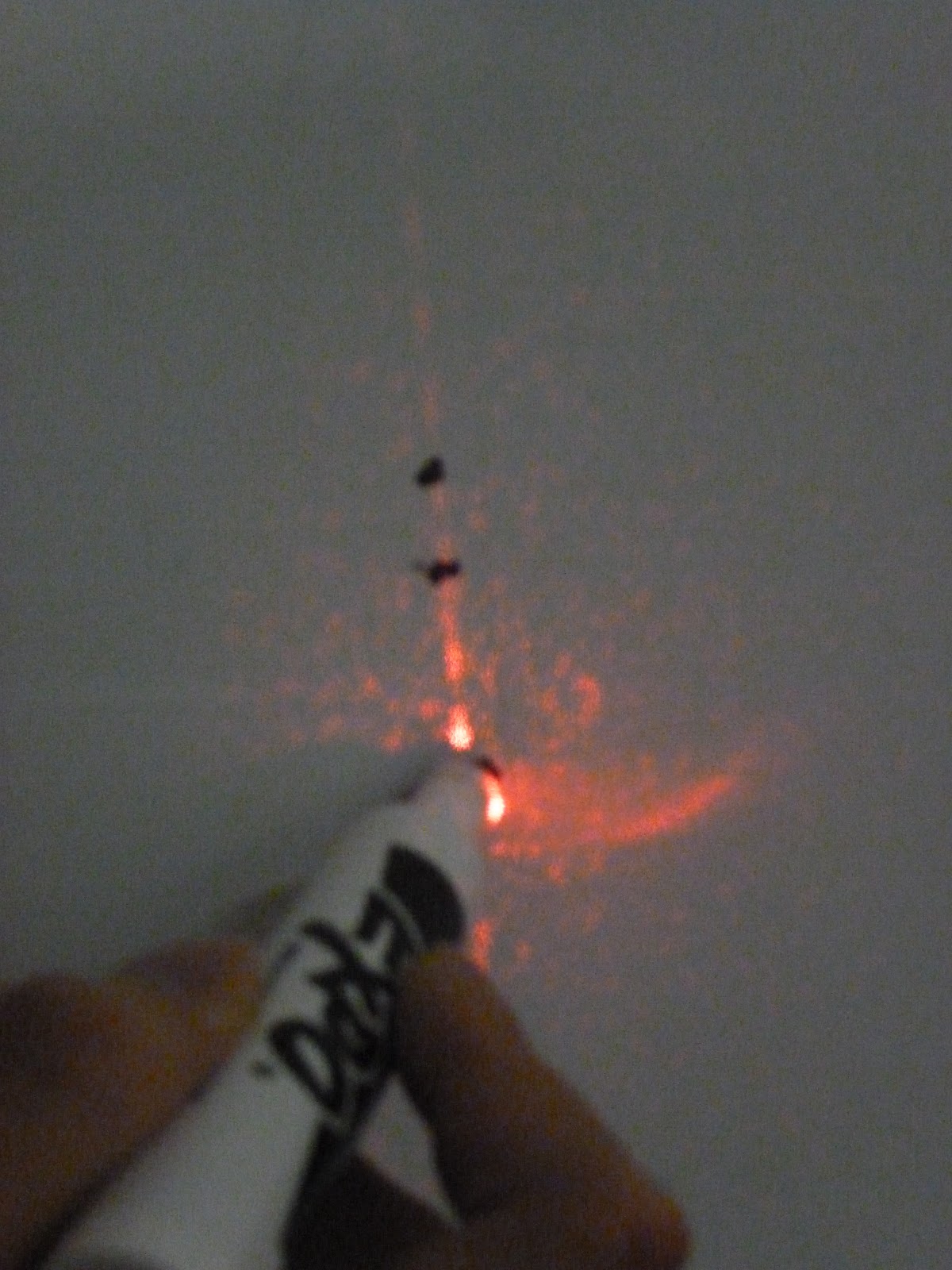
 Figure 3: Measuring the diameter of the hair using a micrometer

Data and Analysis

Table 1

Wavelength,λ (nm)	632.8
Distance,L (cm)	109 ± 1
Distance between 2 fringes,y (cm)	0.8 ± 0.05
Experimental diameter of the hair (μm)	90.0 ± 3
Actual Diameter of the hair (μm)	86.2 ± 1.25
% error (%)	4.41

Conclusion

As shown in table 1, the experimental diameter of the hair was measured to be 90 μm while the actual diameter was 86.2 μm. Therefore, the percent error was very small, and these values were within the uncertainties of each other since the smallest experimental diameter was 87 μm and the largest actual diameter was 87.45 μm.       

Based on the observation of this experiment, light interfered constructively and destructively depending on the distance travelled by each of the secondary light source. At the middle of the light source where both secondary light sources travelled equal distance, the light was the brightest. However there was no light when their distance travelled was a half wavelength difference. Therefore, there was a dark space between 2 bright fringes as shown in figure 2. Since the distance between the lens and the white board was a lot larger than the diameter of the hair, the equation mentioned could be used to compute the diameter of the hair. Otherwise, this equation could not be applied in this case. In addition, the laser beam had to be perpendicular and pass through the hole equally to form the accurate diffraction patter. Despite these disadvantages, the light interference method could accurately measure the diameter of the hair or the width the slits, but the micrometer had more uncertainties in measurement. Yet using the micrometer could be done faster to obtain an approximately accurate result, and there was no need to consider about the distance between the micrometer and the hair.                 

Experiment 10: Lenses

Introduction

The purpose of this experiment was to observe how the image changes based on the object distance. In this experiment, a meter stick, a converging lens, and a socket lamp with filament, a lens holder, and a cardboard. First, the focal length of the lens was determined by measuring the distance between the lens and the focus of the sun rays. Then the object distances varying from 1.5f to 5f were computed using the focal length. These computed distances were used to position the lens distance from the filament. The set up of the apparatus was shown in figure 2. The height of the filament was also measured. After turning the power on to let the light shine through the filament, the cardboard distance from the lens was adjusted till a sharp image was obtained. This image distance and its height were also measured. After recording all these data, the magnification of the lens was computed, and two graphs were constructed to observe the relationship between the image and object distance, and the focal length.  

 Figure 1: Measuring the focal length of the converging lens

Figure 2: Experimental set-up

Figure 3: Image forming through the converging lens

Data and Analysis

Focal length (f) = 9.5 ± 0.25 cm

Table 1: Recorded data of the object and image distances and heights

Object distance as a multiple of f(cm)	Object distance(cm)	Image distance(cm)	Object height(cm)	Image height(cm)	Type of image
5f	47.5 ± 1.25	16.50 ± 0.25	8.80 ± 0.25	3.30 ± 0.25	Inverted, real
4f	38.0 ± 1.00	17.00 ± 0.25		4.40 ± 0.25	Inverted, real
3f	28.5 ± 0.75	18.00 ± 0.25		6.60 ± 0.25	Inverted, real
2f	19.0 ± 0.50	25.50 ± 0.25		14.30 ± 0.25	Inverted, real
1.5f	14.3 ± 0.38	23.25 ± 0.25		16.50 ± 0.25	Inverted, real

Table 2: Comparison of magnification from distance ratios and height ratios

Object distance as a multiple of f(cm)	Md (di/d0)	Mh (hi/h0)	% difference between Md and Mh (%)
5f	0.347 ± 0.011	0.375 ± 0.030	5.10
4f	0.447 ± 0.013	0.500 ± 0.032	7.33
3f	0.632 ± 0.019	0.750 ± 0.036	11.1
2f	1.34 ± 0.04	1.63 ± 0.05	12.6
1.5f	1.63 ± 0.05	1.88 ± 0.06	9.28

Graph 1: Object distance vs. Image distance

Graph 2: Inverse image distance vs. Negative inverse object distance

Conclusion

According to table 1 and graph 1, as the object distance decreased, the image distance increased. Therefore, the image and object distance had inverse relationship as shown in graph 1. However, at 1.5f, even though the object distance decreased, the image distance decreased. This was because the image became dimmer and unclearer as the object distance decreased. Hence, uncertainty became greater since it became harder to see the actual height of the image. Another relationship observed in this experiment was that the image height increased as the object distance decreased. This was because the image distance got smaller. Besides, the image observed was always inverted. Since the image formed by the converging lens was inverted, the image was real. This idea was explained in experiment 9. As shown in table 2, the magnification obtained from distance ratio and height ratio increased as the object distance decreased. This agreed with the observation since the image got larger as the object was nearer to the lens. However, most of these values were not within the uncertainties of each other. This was possibly because the focus was not as accurate as it should have been. Unclear images at small object distances also contributed to this error.

According to graph 2, the inverse image distance and inverse object distance had linear relationship. This relationship actually described the relationship between the image distance, object distance, and the focal length, which was 1/d₀ + 1/d_i = 1/f. The y-intercept 0.08178cm^-1, obtained from the graph was the inverse of the focal length of the lens. By taking the reciprocal of the y-intercept, the graphical focal length was computed to be 12.23cm. However, the measured focal length was 9.5cm. This large difference in focal length was contributed by the image distance at 1.5f. As mentioned earlier, this was the only data set that deviated from the image-object distance relationship. This smaller image distance with larger inverse value lower the slope, hence, smaller y-intercept and larger focal length.
When half of the lens was covered, the image became dimmer since the light passed through the lens was decreased by a factor of 2 due to halved-lens. Besides, as the object distance became closer to the lens, the image size and distance became larger. At 0.5f, there was no image because the image was between the vertex and the focus; hence, the image became virtual.

Experiment 9: Concave and Convex Mirrors

Introduction

                The purpose of this experiment is to understand how images are formed differently in a plane, a concave, and a convex mirror. In this experiment, a concave, a convex, and a plane mirror are used, and the changes in image at different object distances are observed. A light ray diagram corresponding to each case is also constructed to confirm this observed behavior. The magnification of the concave and convex mirrors are also computed using the light ray sketches. 

Figure 1: Convex mirror

Figure 2: Concave mirror

Diagrams

Diagram 1: Light ray diagrams which show how the image in convex mirror changes depending on the object distance

Diagram 2: Light ray diagrams which show how the image in concave mirror changes depending on the object distance

  

Diagram 3: Light ray diagrams which were used to compute magnification of the mirrors

Data

Table 1: Comparison of magnification

Magnification ratio	Magnification of the mirror
	Convex	Concave
hi/h0	0.318 ± 0.024		-0.339 ± 0.009
di/d0	-0.304 ± 0.023		0.297 ± 0.008

Sample Calculation

Conclusion

                According to the experimental observation, the image formed by the convex mirror appeared to be always smaller than the object, and it is always upright. As the object was moved further away from the mirror, the image also appeared smaller, and it became larger as the object was closer. The reason that the image appeared as it was, was illustrated by diagram 1. When a ray of light hit the convex mirror, the light was reflected, and these reflected rays were appeared as they were radiated from the image. Since the reflected rays of light did not pass through the image, the image was a virtual image. Based on this observation, it was concluded that a convex mirror always formed upright, virtual image which were smaller than the object.

                As for concave mirror, the image was observed to be inverted when the object was placed further away from the mirror. As the object got closer, at a certain distance, the image became erect. This was because the object distance determined how the image was formed. As shown in diagram 2, when the object distance was larger than the focal length, the image was always inverted. Once the object distance equaled the radius of curvature, the object distance and the image distance became the same, but the orientation was different. But the image disappeared if the object was at the focal length since the image was at infinity. On the other hand, when the object distance was smaller than the focal length, the image was always virtual and erect since the actual light rays did not pass through the image. Therefore, the observation was agreed with the light ray sketch illustrated in figure 2.

                In plane mirror, the image and the object always showed the same size and distance no matter where the object distance was. In addition, the images formed in plane mirror were virtual and erect images.

                In the last part of the experiment were the mirror magnification were to be computed based on the sketch, it was found that the magnification computed from the object and image distance ratio was agreed with that from the height ratio as shown in table 1. However, their signs were opposite. This was because, in convex mirror, the image was a virtual image, but both the object and image distances were erected. On the other hand, in concave mirror, the image is real and inverted. Therefore, the image height was negative.  These sign determinations were shown in diagram 3.  

Experiment 7: Standing Electromagnetic Waves: Determination of the dimensions of a microwave, the rate of oscillating photons, and the pressure of photons on the microwave

Introduction

                The purpose of this experiment was to understand the standing waves created by electromagnetic waves, to solve the possible dimensions for microwaves by using standing waves concept, and to compute the rate of oscillating photons and the pressure exerted on the walls of microwaves by these photons.

                This experiment was conducted using a microwave, a bag of marshmallows, a paper, a cup of 100g of water, and a multimeter. Marshmallows were uniformly spread out on a paper and were microwaved for a few seconds to observe the standing wave pattern created by the electromagnetic waves. Half of the wavelength was obtained by measuring crest to crest of the marshmallows. The dimensions of the microwave were also recorded. Then 100 g of water was microwaved for 30s, and the change in temperature was recorded. The frequency and the dimensions of the microwave were computed by using the measured half wavelength. Also, the total energy content, the rate of photons oscillating in the microwave, and the pressure exerted by these photons on each dimension of the microwave were computed by using the concepts of heat transfer, Planck relation, and energy and momentum in electromagnetic waves. The following equations describing these concepts were used.

Heat transfer:                                                       Q=mc∆T                             (1)

Planck Relation:                                                   E=hc/λ                                          (2)

Energy and Momentum in electromagnetic waves:  I=P/A=p_radc                         (3) 

Figure 1: Marshmallows before being microwaved

Figure 2: Measuring water temperature after microwaving for 30s

 Video 1: Microwaving marshmallows: Marshmallows formed 3-dimensional standing waves pattern as it was being microwaved.

Data and Analysis

Table-1: Various recorded and calculated values from this experiment

Experimental measurements		Calculated values
λ/2(cm)	12.0 ± 1.0	ƒ(GHz)		1.25 ± 0.104
Length(cm)	35.0 ± 1.0	Length(cm)		36 ± 3.0
Width(cm)	35.0 ± 1.0	Width(cm)		36 ± 3.0
Height(cm)	23.0 ± 1.0	Height(cm)		20.0 ± 2.0
Amplitude(cm)	10.0 ± 1.0	Q(J)		15500 ± 466
Masswater(g)	100.0 ± 3.0	Ephotons(J)		(8.29 ± 0.691)x10-25
Tempi(˚C)	20.0 ± 0.05	Rate(photons/s)		(6.23 ± 0.833)x1026
Tempi(˚C)	57.0 ± 0.05	Power(W)		516 ± 54
Time(s)	30.0 ± 3.0	pphotons(μPa)	35x35	14.0 ± 2.72
			35x23	21.4 ± 5.77

Figure 3: Marshmallows after being microwaved: The second image showed that the places with most marshmallows were antinodes and those with very few marshmallows were nodes. 

Calculations of uncertainties

Conclusion

                In this experiment, the wavelength of the standing waves created by microwave was considered to be 24cm since the length from crest to crest of the marshmallows shown in figure 3 were 12cm apart. According to table 1, the computed dimensions of the microwave were 36x36x20 which were within the uncertainties of the measured values 35x35x23. The computed length and width of the microwave were greater than that of the measured values. This was because it was assumed that in each dimension of the paper, there was one and a half wave. In fact, as shown in figure 3, there was less than one and a half wave. Hence, the possible length and width should have been smaller than 36x36. In addition, the amplitude of the standing wave was measured to be 10cm which was a half of the height of the microwave. Therefore, the height was considered to be 20cm, but it was only an approximation. Therefore, it had a large uncertainty. If the height could not be approximated, the height of the microwave could possibly be any height approximately equal to or greater than 10cm in this particular case. If it was a lot lower than 10cm, standing waves will not possible be observed due to compression on marshmallows by the height limit.

                According to table 1, the frequency of the standing microwave was 1.25GHz, and it was computed by using the relationship between the speed of light, the frequency, and the measured wavelength. The result was within the normal range, 1-300GHz*, of the frequency emitted from a microwave oven. Besides, the heat content which was 15500J was also computed by using the measured mass and the temperature change of 100g of water. Moreover, computation revealed that there were (6.23 ± 0.833)x10²⁶ photons oscillating in the microwave in a second. These photons exerted 14 to 21.4 μPa on each wall of the microwaves. This result was obtained by using equation 3 described in the introduction. Lastly, the power of the microwave was experimentally calculated to be 516W, which agreed with the power produced by a typical consumer microwave ranging from 400W to 1200W*.

*source: Frequency of a Microwave, Power of a Microwave