Experiment 7: Standing Electromagnetic Waves: Determination of the dimensions of a microwave, the rate of oscillating photons, and the pressure of photons on the microwave

Introduction

                The purpose of this experiment was to understand the standing waves created by electromagnetic waves, to solve the possible dimensions for microwaves by using standing waves concept, and to compute the rate of oscillating photons and the pressure exerted on the walls of microwaves by these photons.

                This experiment was conducted using a microwave, a bag of marshmallows, a paper, a cup of 100g of water, and a multimeter. Marshmallows were uniformly spread out on a paper and were microwaved for a few seconds to observe the standing wave pattern created by the electromagnetic waves. Half of the wavelength was obtained by measuring crest to crest of the marshmallows. The dimensions of the microwave were also recorded. Then 100 g of water was microwaved for 30s, and the change in temperature was recorded. The frequency and the dimensions of the microwave were computed by using the measured half wavelength. Also, the total energy content, the rate of photons oscillating in the microwave, and the pressure exerted by these photons on each dimension of the microwave were computed by using the concepts of heat transfer, Planck relation, and energy and momentum in electromagnetic waves. The following equations describing these concepts were used.

Heat transfer:                                                       Q=mc∆T                             (1)

Planck Relation:                                                   E=hc/λ                                          (2)

Energy and Momentum in electromagnetic waves:  I=P/A=p_radc                         (3) 

Figure 1: Marshmallows before being microwaved

Figure 2: Measuring water temperature after microwaving for 30s

 Video 1: Microwaving marshmallows: Marshmallows formed 3-dimensional standing waves pattern as it was being microwaved.

Data and Analysis

Table-1: Various recorded and calculated values from this experiment

Experimental measurements		Calculated values
λ/2(cm)	12.0 ± 1.0	ƒ(GHz)		1.25 ± 0.104
Length(cm)	35.0 ± 1.0	Length(cm)		36 ± 3.0
Width(cm)	35.0 ± 1.0	Width(cm)		36 ± 3.0
Height(cm)	23.0 ± 1.0	Height(cm)		20.0 ± 2.0
Amplitude(cm)	10.0 ± 1.0	Q(J)		15500 ± 466
Masswater(g)	100.0 ± 3.0	Ephotons(J)		(8.29 ± 0.691)x10-25
Tempi(˚C)	20.0 ± 0.05	Rate(photons/s)		(6.23 ± 0.833)x1026
Tempi(˚C)	57.0 ± 0.05	Power(W)		516 ± 54
Time(s)	30.0 ± 3.0	pphotons(μPa)	35x35	14.0 ± 2.72
			35x23	21.4 ± 5.77

Figure 3: Marshmallows after being microwaved: The second image showed that the places with most marshmallows were antinodes and those with very few marshmallows were nodes. 

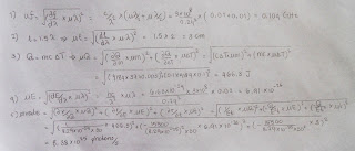
Calculations of uncertainties

Conclusion

                In this experiment, the wavelength of the standing waves created by microwave was considered to be 24cm since the length from crest to crest of the marshmallows shown in figure 3 were 12cm apart. According to table 1, the computed dimensions of the microwave were 36x36x20 which were within the uncertainties of the measured values 35x35x23. The computed length and width of the microwave were greater than that of the measured values. This was because it was assumed that in each dimension of the paper, there was one and a half wave. In fact, as shown in figure 3, there was less than one and a half wave. Hence, the possible length and width should have been smaller than 36x36. In addition, the amplitude of the standing wave was measured to be 10cm which was a half of the height of the microwave. Therefore, the height was considered to be 20cm, but it was only an approximation. Therefore, it had a large uncertainty. If the height could not be approximated, the height of the microwave could possibly be any height approximately equal to or greater than 10cm in this particular case. If it was a lot lower than 10cm, standing waves will not possible be observed due to compression on marshmallows by the height limit.

                According to table 1, the frequency of the standing microwave was 1.25GHz, and it was computed by using the relationship between the speed of light, the frequency, and the measured wavelength. The result was within the normal range, 1-300GHz*, of the frequency emitted from a microwave oven. Besides, the heat content which was 15500J was also computed by using the measured mass and the temperature change of 100g of water. Moreover, computation revealed that there were (6.23 ± 0.833)x10²⁶ photons oscillating in the microwave in a second. These photons exerted 14 to 21.4 μPa on each wall of the microwaves. This result was obtained by using equation 3 described in the introduction. Lastly, the power of the microwave was experimentally calculated to be 516W, which agreed with the power produced by a typical consumer microwave ranging from 400W to 1200W*.

*source: Frequency of a Microwave, Power of a Microwave    

Experiment 6: Length of the Pipe

Introduction

The purpose of this experiment is to determine the length of an open pipe by using sound waves. The experiment was conducted using an open pipe, a microphone, Logger Pro, a guitar, and two tuning forks. In part 1, an open pipe with unknown length was spun with a speed till a clear tone was heard. The microphone was put near the spinning pipe, and the sound wave was recorded by using Logger Pro. This process was repeated with a greater spinning speed that gave the next level of tone.

Data and Analysis

Table 1: Data recorded from spinning the open pipe

Spinning Speed	ω(rad/s)	ƒ(Hz)	λ(m)
Low	3859 ± 0.4736	614.2 ± 0.07538	0.558 ± 0.0000679
Fast	5068 ± 1.016	806.6 ± 0.1617	0.425 ± 0.0000845

Table 2: Comparison of the length of the open pipe obtained from 2 data sets

Spinning Speed	Lexp(m)	Lact(m)	% Error(%)
Low	0.837 ± 0.000102	0.80 ± 0.05	4.6
Fast	0.850 ± 0.000169		6.3

Figure 1: Calculation of the length of the open pipe

Conclusion

                In this experiment, the length of the pipe was computed by using the concept of the fundamental frequency and its harmonics. Since it was an open pipe, it had the wavelength that was twice of the length of the pipe. Since the second frequency produced the next tone after the first, the second frequency had a half wavelength longer than the wavelength of the first frequency. By using this relationship, as shown in figure 1, n value was calculated, and the length of the pipe was found. As shown in table-1, the lengths of the open pipe obtained from two sets of data were 0.837m and 0.850m. This resulted in a percent error of 4.6% and 6.3%. Even though the experimental results were not within the uncertainties of each other, these values were within the uncertainty of the actual length of the pipe. Table 1 showed that the experimental lengths were greater than that of the actual length. This was possibly due to the fact that the pipe stretched when it was spun. Since the pipe had tension, the pipe could stretch approximately 4cm longer. 

Experiment 5: Introduction to Sound

Introduction

                The purpose of this experiment is to understand the sound waves by examining their characteristics such as their wave pattern, frequencies, amplitudes, periods, and wavelengths. Simple relationships between these characteristics are used to compute and confirm the experimental results.

                This experiment was conducted using a tuning fork, a microphone, and a Lab Pro. The experiment was set up as shown in figure 1. For the first part of this experiment, a pressure vs. time graph of a person saying “AAA” into the microphone was constructed using Logger Pro. This procedure was repeated with a different person saying “AAA.” Once the graphs were constructed, a comparison between these graphs were made and analyzed. As a second part, a pressure vs. time graph of a tuning fork stricken by a soft object was constructed, and this was repeated with the same tuning fork with a different loudness. The graph was analyzed, and a comparison was made. Finally, the sound waves produced by a human voice and a tuning fork were compared and were analyzed.

Figure 1: Experimental set-up

Data and Analysis

Table 1: Comparison between the sound waves produced by first and second person

Person	Period(s)	Frequency(Hz)	Wavelength(m)	Amplitude	# of waves in 0.03s
1	0.0085 ± 0.0005	118 ± 6.9	2.9 ± 0.17	0.850 ± 0.005	3.5
2	0.0075 ± 0.0005	133 ± 8.9	2.6 ± 0.17	0.078 ± 0.005	4

Table 2: Comparison between the sound waves produced by a tuning fork with different loudness

Person	Period(s)	Frequency(Hz)	Wavelength(m)	Amplitude	# of waves in 0.03s
1	0.0040 ± 0.0005	250 ± 31.3	1.4 ± 0.17	0.101 ± 0.005	7.5
2	0.0040 ± 0.0005	250 ± 31.3	1.4 ± 0.17	0.012 ± 0.005	7.5

Figure 2: Sound Pressure vs. Time of a human voice (1) 

Figure 3: Sound Pressure vs. Time of a human voice (2)

Figure 4: Sound Pressure vs. Time of a tuning fork (1)

Figure 5: Sound Pressure vs. Time of a tuning fork (2) 

Figure 6: Sound Pressure vs. Time of a human voice with a time frame of 0.3s

Summary

               The sound wave produced by human voice in this experiment was a periodic wave because the same pattern was repeated in a measured time frame. For instance, as shown in figure 2, the wave pattern from 0.0s to 0.0085s repeatedly showed up for 3 and a half times in 0.03s. This was confirmed by dividing the total time taken by the period, and it also resulted in 3.5 waves. Since one complete wave pattern was seen in the first 0.0085s, it was taken as the period of these waves. Hence, frequency turned out to be 118Hz since the frequency was the reciprocal of the period. The wavelength was also computed to be 2.89m, where v was equal to the speed of the sound. Besides, figure 2 showed that the power was changing from minimum 1.8 to 3.5 units. Therefore, the power amplitude was determined to be half of the difference between these 2 values, which was 0.85. If the sample was 10 times as long, these characteristics would probably not change. Perhaps 10 times as many waves would be shown in 0.3s. In figure 6, the sound wave of the human voice in 0.3s time frame was recorded. However, the voice loudness, tones, and frequencies had all changed.

In comparison to figure 2 and 3, figure 2 had larger period since the period in figure 3 was about 0.0075s and that in figure 2 was 0.0085s. Therefore, the frequency of the first person was smaller, hence, smaller pitched. Since they had different frequencies, their wavelengths also differed as shown in table 1. Their amplitude differed because they had different loudness. The first person’s voice was louder than the second one; hence, the first one had higher amplitude. In addition, figure 3 showed 4 waves in 0.03s whereas figure 2 showed only 3 and a half waves in the same period of time. All of these differences were shown in table 1.

In figure 4 and 5, both of the graphs were created by a sound from the same tuning fork but with different loudness. Since both of these were of the same tuning fork, they were expected to produce the same wavelength and frequencies. This was confirmed by these experimental results shown in figure 4 and 5. However, they produced amplitudes with a difference in the order of 10 as shown in table 2. This was because the loudness of the sound was dependent on its amplitude. In the second trial with the tuning fork, the sound was made softer by simply striking it softer, so it produces lower sound. Since the first trial created louder voice than the second, it should have larger amplitude. Therefore, the experimental results were consistent.

By comparing all of the graphs in figure 2 to 5, it was seen clearly that human voice was not a simple sinusoidal wave, and it was not smooth. However, the tuning fork was. No matter the sound of the tuning fork was made louder or softer, it produced the same frequency and wavelength, but this was not true for human voice. The time frame 0.03s used in this experiment was very short. This revealed that sound waves were really small. In real life, perhaps only the images from television screen can show several frames in this time frame.  

Experiment 4: Standing Waves

Introduction

                The purpose of this experiment is to investigate the behavior of standing waves caused by an external force to initiate a transverse wave on a string. Standing wave occurs when an original wave and a reflected wave superpose. Standing waves have constant wave pattern, and the amplitude of the points on the wave are changing. The only points that are not changing in a standing wave are nodes. Node is half of the wavelength. The relationship between the length of the string (L), number of half wavelengths or loops (n), and wavelength (λ) is indicated by

L=nλ/2                                  (1)

 As found in experiment 3, frequency, wavelength, and velocity of a transverse wave in a string is related according to this equation.

ƒ = v/λ                                  (2)

And the velocity of a transverse wave can be obtained by

v=√(T/μ)                                (3)

where v is velocity or wave speed, T represents tension, and μ indicated mass density.

                The experiment was conducted using various apparatus such as variable frequency wave driver, function generator, 200g and 50g weight hanger, table clamps, rod, pendulum clamp, pulley, multimeter, and a meter stick. The mass and length of the string were recorded to determine its mass density, μ. One end of the string was attached to a 200g weight hanger, and the other end was tied to the clamp. The length or distance between each end was measured to be 1.2m. The string wave driver which was connected with the function driver was put 10cm away from the pendulum clamp. The function generator was set to 5.0 voltages, and the frequency was adjusted to get a certain number of loops. Frequencies with respective number of loops were recorded. The procedure was repeated using 50g weight hanger in place of 200g. The wavelength and velocity were computed based on the data. Two graphs were constructed, and the velocity obtained from the graph was compared with that from computation. 

Figure 1: The set-up of the apparatus to measure the frequency of standing waves with various loops  

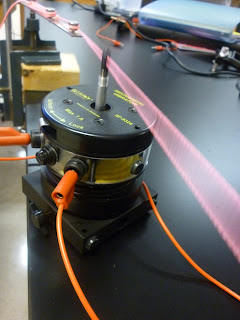
Figure 2: Wave driver that helps to create transverse waves

Data and Analysis

L=1.2 ± 0.05m, m_rope =1.47 ± 0.005g,

      1)  m_tension = 200 ± 0.5g

      2)  m_tension = 50 ± 0.5g

Table1: Recorded frequency, nodes, and calculated wavelength, velocity for 200g of weight

n # of loops	ƒ1 (Hz)	ƒn = nƒ1 (Hz)	# of nodes	λ (m)	velocity(m/s)
1	18 ± 0.5	18 ± 0.5	2	2.40 ± 0.10	40.0 ± 0.84
2	37 ± 0.5	36 ± 1.0	3	1.20 ± 0.05
3	56 ± 0.5	54 ± 1.5	4	0.800 ± 0.033
4	76 ± 0.5	72 ± 2.0	5	0.600 ± 0.025
5	95 ± 0.5	90 ± 2.5	6	0.480 ± 0.020
6	114 ± 0.5	108 ± 3.0	7	0.400 ± 0.017
7	133 ± 0.5	126 ± 3.5	8	0.343 ± 0.014

Table2: Recorded frequency, nodes, and calculated wavelength, velocity for 50g of weight

n # of loops	ƒ2 (Hz)	ƒn = nƒ1 (Hz)	# of nodes	λ (m)	velocity(m/s)
1	8 ± 0.5	8 ± 0.5	2	2.40 ± 0.10	20.0 ± 0.43
2	19 ± 0.5	16 ± 1.0	3	1.20 ± 0.05
3	28 ± 0.5	24 ± 1.5	4	0.800 ± 0.033
4	38 ± 0.5	32 ± 2.0	5	0.600 ± 0.025
5	48 ± 0.5	40 ± 2.5	6	0.480 ± 0.020
6	58 ± 0.5	48 ± 3.0	7	0.400 ± 0.017
7	70 ± 0.5	56 ± 3.5	8	0.343 ± 0.014

Table 3: Ratio of frequencies from table 1 and 2

n # of loops	1	2	3	4	5	6	7	Average
ƒ1 / ƒ2	2.3	1.9	2.0	2.0	2.0	2.0	1.9	2.0

Table 4: Comparison of ratio of wave speeds from computation and graphing

Methods	v1/v2
Computation	2.00
Graph	1.892

Graph 1: Frequency vs. 1/wavelength (200g)

Graph 2: Frequency vs. 1/wavelength (50g)

Calculations of uncertainties

      1)  λ = 2L/n

uλ = √(dλ/dL x uL)² = √(2/n x uL)²

     = √(2/1 x 0.05)² = 0.10 m

      2)  T = mg

uT = √(dT/dm x um)² = √(g x um)²

     = √(9.8 x 0.0005)² = 0.0049 N

      3)  μ = m/L

uμ = √[(∂μ/∂m x um)² + (∂μ/∂L x uL)²] = √[1/L x um)² + (-m/L² x uL)²]

      = √[1/1.20 x 0.000005)² + (-0.00147/1.2² x 0.05)²] = 0.0000512 kg/m

      4)  v = √(T/μ)

uv = √[(∂v/∂T x uT)² + (∂v/∂μ x uμ)²] = √[(0.5/(μ√(T/μ)) x uT)² + (-0.5T/(μ²√(T/μ)) x uμ)²]

     = √[(0.5/(0.001225√(1.96/0.001225)) x 0.0049)² + (-0.5 x 1.96/(0.001225²√(1.96/0.001225)) x 0.0000512)²]

     = √(0.0025 + 0.69875)

     =0.837 m/s

Conclusion

As shown in table 1 and graph 1, the wave speeds from computation and from the graph were approximately 40.0 m/s and 46.04 m/s. Even though these values did not agree within the uncertainties, these results were very similar. In same manner, the wave speeds were 20.0m/s and 24.34 m/s respectively when 50g hanging mass was used. These results were shown in table 2 and graph 2. Again, these values were not within the uncertainties. In column 2 and 3 of table 1 and 2, the comparison between the recorded frequencies and the computed frequencies were shown. The frequencies on column 3 were a factor of the first recorded frequency, and these should have been the same with the recorded frequencies. However, column 2 and 3 values were not agreed within the uncertainties. As wavelength decreased, larger deviation from the recorded frequencies was observed.

According to table 4, the ratios of wave speed computed based on data and graph were approximately 2. Even though the ratios were not exactly the same, they highly agreed with each other. This result was confirmed by the equation 3 mentioned in the introduction. Since velocity was proportional to square root of tension, velocity had to decrease by a factor of 2 when tension decreased by a factor of 4.  In table 3, it was shown that the ratio of ƒ₁ and ƒ₂ were approximately 2. Even though the ratio changed a little for different loop numbers, the ratio maintained fairly constant. This was reasonable because frequency and velocity were directly proportional according to the equation 2. Therefore, as velocity increased by a factor of 2, so did the frequency.

There were a lot of possible experimental errors that could cause the above compared values not to agree within uncertainties. First, there was an inaccuracy in adjusting frequencies to obtain an exact number of loops. As the frequency was raised to higher value to obtain more nodes, the wave became harder to visible. Another factor influenced the experimental result was that the loop should be counted starting from the wave driver, but the loop was counted from the point of the clamp where the string was tied. This was shown in figure 2. If the number of loops was counted from the wave driver, the frequency could change. Therefore, these factors could contribute to inaccurate values of frequency which then led to inaccurate wave speed. In addition, the hanging mass did not remain stable throughout the experiment. This vibration in hanging mass could also cause a variation of tension in the string. Approximation in reading the length of the string also contributed to these errors. All of these led to inaccuracy in calculations of wavelength and velocities.